Sample Code of VMS stabilizaiton in mixed form 2D Stokes: Lid-Driven Cavity
written by L. Zhu and A. Masud (2019).
Contents
This script is served to illustrate the general paradigm for implementation of Variational Multiscale (VMS) method for partial differential equations (PDE) with intrinsic instabilities. Specifically, a mixed form of incompressible Stokes flow is solved with equal order interpolation (linear quadrilateral element) of velocity and pressure fields.
For the extension of the VMS method for incompressible Navier-Stokes equations and isothermal turbulence model for Large Eddy Simulation (LES), interested readers are referred to Masud & Khurram 2006 and Masud & Calderer 2011.
clearvars; close all;
Mesh generation
Mesh generation:  stretched Q4 element
res_el_1D = 40; % Number of elements per dimension
res_node_1D = res_el_1D + 1; % Number of nodes perdimension
ndf = 3; % Number of degrees of freedom per node (u1, u2, p)
nel = 4; % Number of nodes per element (Q4)

x_unif = linspace(0, res_el_1D, res_node_1D) / res_el_1D; % 1D coordinates for uniform mesh
[Ycoord, Xcoord] = meshgrid(x_unif, x_unif); % Generate spatial grid

nnode = res_node_1D ^ 2; % Number of nodes for the 2D domain
node_num = linspace(1, nnode, nnode); % Node numbering in vector form
node_num_mtx = reshape(node_num, [res_node_1D, res_node_1D]); % Node numbering in matrix form
Gaussian Quadrature Rules
3 integration points in each dimension
wght_1D = [5/9, 8/9, 5/9]; % weights of 1D integration rule
gp_loc_1D = [-sqrt(3/5), 0, sqrt(3/5)]; % location of 1D integration rule
gp_2D = zeros(9, 3); % location and weight of 2D integration rule: 9 points
k = 0;
for i = 1:3
    for j = 1:3
        k = k + 1;
        gp_2D(k, :) = [gp_loc_1D(i), gp_loc_1D(j), wght_1D(i)*wght_1D(j)];
    end
end
Stabilized Weak Form
Strong Form

Stabilized Weak Form

Stabilization Tensor
R_global = zeros(nnode*ndf); % Initialize the global residual (zero in this test case)
K_global = zeros(nnode*ndf, nnode*ndf); % Initialize the global consistent tangent matrix
xl = zeros(2, 4); % Initialize the element-wise nodal coordinates matrix
Loop Over the Elements
for j = 1:res_el_1D
    for i = 1:res_el_1D
        xl(1,:) = [x_unif(i), x_unif(i+1), x_unif(i+1), x_unif(i)]; % Fetch x coordinate
        xl(2,:) = [x_unif(j), x_unif(j), x_unif(j+1), x_unif(j+1)]; % Fetch y coordinate
        node_el = [node_num_mtx(i,j), node_num_mtx(i+1,j), node_num_mtx(i+1,j+1), node_num_mtx(i,j+1)]; % Element connectivity
Numerical Quadrature for VMS stabilizaiton tensor 
        Tau_dnm = zeros(ndf-1, ndf-1); % Denominator
        Tau_nmr = 0.0; % Numerator
        for l = 1 : 9 % Loop over quadrature points
            % shape function and its derivatives at Gaussian point l
            [shg, ~, jcb] = shp_bbl_Q4(xl, gp_2D(l,1:2));
            bbl = shg(3,5); bbl1 = shg(1,5); bbl2 = shg(2,5);
Denominator of Tau: 
            Tau_dnm = Tau_dnm + [2.0*bbl1^2+bbl2^2, bbl1*bbl2;
                                 bbl1*bbl2,         bbl1^2+2.0*bbl2^2] * jcb * gp_2D(l,3);
Numerator of Tau: 
Tau_nmr = Tau_nmr + bbl * jcb * gp_2D(l,3);
        end
        Tau_hat = inv(Tau_dnm) * Tau_nmr; % Compute the stabilizaiton tensor
Numerical Quadrature for Consistent Tangent
        k_local = zeros(nel*ndf, nel*ndf);
        for l = 1 : 9
            % shape function and its derivatives at Gaussian point l
            [shg, shgs, jcb] = shp_bbl_Q4(xl, gp_2D(l,1:2));
            % location of Gaussian point in physical coordinates
            x_GP = shg(3,1:4) * xl(1,:)';
            y_GP = shg(3,1:4) * xl(2,:)';
            % Enrich the fine-scale solution with bubble basis
            Tau11 = Tau_hat(1,1) * shg(3,5); Tau22 = Tau_hat(2,2) * shg(3,5);
            for a = 1 : nel
                Na  = shg(3,a); Na1 = shg(1,a); Na2 = shg(2,a); Na12 = shgs(3,a);
                for b = 1 : nel
Nb = shg(3,b); Nb1 = shg(1,b); Nb2 = shg(2,b); Nb12 = shgs(3,b);
Galerkin diffusion: 
                    k_Diff_Gal = [Na1*Nb1*2.0 + Na2*Nb2, Na2*Nb1,               0;
                                  Na1*Nb2,               Na1*Nb1 + Na2*Nb2*2.0, 0;
                                  0,                     0,                     0];
Galerkin duality of incompressibility: 
                    k_C_Gal = [0,   0,         -Na1*Nb;
                               0,   0,         -Na2*Nb;
                               Na*Nb1, Na*Nb2, 0];
VMS Terms: 
                    k_VMS = [-Na12*Tau22*Nb12, 0,                Na12*Tau22*Nb2;
                             0,                -Na12*Tau11*Nb12, Na12*Tau11*Nb1;
                             -Na2*Tau22*Nb12,  -Na1*Tau11*Nb12,  Na1*Tau11*Nb1+Na2*Tau22*Nb2];
                    % Element-wise consistant tangent
                    k_gp = k_Diff_Gal + k_C_Gal + k_VMS;
                    k_local((a-1)*ndf+1:a*ndf,(b-1)*ndf+1:b*ndf) = ...
                        k_local((a-1)*ndf+1:a*ndf,(b-1)*ndf+1:b*ndf) + k_gp * jcb * gp_2D(l,3);
                end
            end
        end
Assembly The Global Consistent Tangent
        for a = 1:nel
            for b = 1:nel
                K_global(node_el(a)*ndf-2:node_el(a)*ndf, node_el(b)*ndf-2:node_el(b)*ndf) = ...
                    K_global(node_el(a)*ndf-2:node_el(a)*ndf, node_el(b)*ndf-2:node_el(b)*ndf) + ...
                    k_local(a*ndf-2:a*ndf,b*ndf-2:b*ndf);
            end
        end
    end
end
Boundary Condition: Lid-Driven Cavity
No-slip Dirichlet BCs on the bottom ( ), left (
 ) and right (
 )
)
Prescribed velocity on the top ( ):
):  and
and  .
.
DOF_list = linspace(1, nnode*ndf, nnode*ndf); % Global DOF list
DOF_list_mtx = reshape(DOF_list, [3, nnode]); % Global DOF list matrix: ndf by #nodes

BC_mask_mtx = zeros(size(DOF_list_mtx)); % Mask for the slots with Dirichlet BCs
BC_mask_mtx(1:2,node_num_mtx([1,end],:)) = 1; % left and right wall
BC_mask_mtx(1:2,node_num_mtx(:,[1,end])) = 1; % bottem and top wall
BC_mask_mtx(3,node_num_mtx(1,1)) = 1; % Fixed pressure at (0,0) to remove constant pressure mode
BC_mask = reshape(BC_mask_mtx, [nnode*ndf, 1]); % mask vector

idx_BC = find(BC_mask>0.5); % indices of DOFs that has Dirichlet BC
idx_sol = find(BC_mask<0.5); % indices of unknown DOFs

BC_val_mtx = zeros(size(DOF_list_mtx)); % Boundary Values
BC_val_mtx(1,node_num_mtx(:,end)) = 1.0; % Unit horizontal velocity on the top
BC_val = reshape(BC_val_mtx, [nnode*ndf, 1]);
Static Condenstaion (Guyan Reduction)
uvp_global = BC_val;
uvp_global(idx_sol) = K_global(idx_sol, idx_sol) \ (R_global(idx_sol) - K_global(idx_sol, idx_BC) * uvp_global(idx_BC));
Visualization of the solution
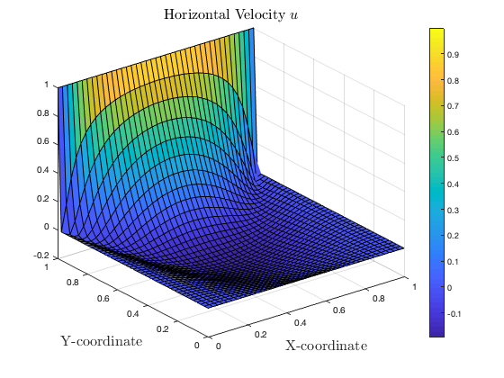
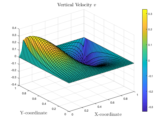
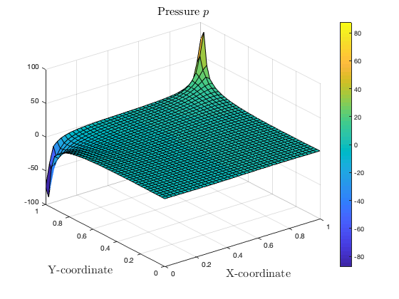
u_gl = reshape(uvp_global(DOF_list_mtx(1,:)), [res_node_1D, res_node_1D]);
v_gl = reshape(uvp_global(DOF_list_mtx(2,:)), [res_node_1D, res_node_1D]);
p_gl = reshape(uvp_global(DOF_list_mtx(3,:)), [res_node_1D, res_node_1D]);

figure;
surf(Xcoord, Ycoord, u_gl);
xlabel('X-coordinate', 'FontSize', 16, 'Interpreter','latex');
ylabel('Y-coordinate', 'FontSize', 16, 'Interpreter','latex');
title('Horizontal Velocity $u$', 'FontSize', 16, 'Interpreter','latex');
colorbar;

figure
surf(Xcoord, Ycoord, v_gl);
xlabel('X-coordinate', 'FontSize', 16, 'Interpreter','latex');
ylabel('Y-coordinate', 'FontSize', 16, 'Interpreter','latex');
title('Vertical Velocity $v$', 'FontSize', 16, 'Interpreter','latex');
colorbar;

figure
surf(Xcoord, Ycoord, p_gl);
xlabel('X-coordinate', 'FontSize', 16, 'Interpreter','latex');
ylabel('Y-coordinate', 'FontSize', 16, 'Interpreter','latex');
title('Pressure $p$', 'FontSize', 16, 'Interpreter','latex')
colorbar;

% figure
% quiver(Xcoord, Ycoord, u_gl, v_gl);
% startx = x_streched';
% starty = ones(size(startx))*0.5';
% streamline(Xcoord, Ycoord, u_gl, v_gl, startx, starty)
% xlim([-0.1, 1.1]); ylim([-0.1, 1.1]);
% xlabel('X-coordinate', 'FontSize', 16, 'Interpreter','latex');
% ylabel('Y-coordinate', 'FontSize', 16, 'Interpreter','latex');
Shape functions and bubble function and their derivatives for Q4 elements
bubble function:
% input : xl(2,4)   nodal coordinates of the element
% input : gp(2)     location of Gaussion points
% output: shg(3,5)  shape function and its derivatives
% output: shg2(3,5) 2nd order derivatives of shape functions
% output: jcb       jacobian
function [shg, shgs, jcb] = shp_bbl_Q4(xl, gp)
    shg = zeros(3, 5);
    shgs = zeros(3, 4);
    x_el = xl(1,2) - xl(1,1); % x2 - x1
    y_el = xl(2,4) - xl(2,1); % y4 - y1
    jcb = x_el * y_el / 4; % affine elements only
    xi = gp(1); eta = gp(2);
    % shape functions
    shg(3,1) = 0.25 * (1 - xi) * (1 - eta);
    shg(3,2) = 0.25 * (1 + xi) * (1 - eta);
    shg(3,3) = 0.25 * (1 + xi) * (1 + eta);
    shg(3,4) = 0.25 * (1 - xi) * (1 + eta);
    shg(3,5) = (1 - xi^2) * (1 - eta^2);
    % x derivative
    shg(1,1) = 0.25 * (-1 + eta);
    shg(1,2) = 0.25 * ( 1 - eta);
    shg(1,3) = 0.25 * ( 1 + eta);
    shg(1,4) = 0.25 * (-1 - eta);
    shg(1,5) = -2 * xi * (1 - eta^2);
    % y derivative
    shg(2,1) = 0.25 * (-1 + xi);
    shg(2,2) = 0.25 * (-1 - xi);
    shg(2,3) = 0.25 * ( 1 + xi);
    shg(2,4) = 0.25 * ( 1 - xi);
    shg(2,5) = -2 * eta * (1 - xi^2);
    % xx derivative
    % yy derivative
    % xy derivative
    shgs(3,1:4) = [0.25, -0.25, 0.25, -0.25] / jcb; % affine element only
    % physical derivative
    shg(1,:) = shg(1,:) * 2 / x_el; % affine element only
    shg(2,:) = shg(2,:) * 2 / y_el; % affine element only
end